World Pipelines - March 2020

63 / 100

Predicting model performance
Assigning performance to these models can be difficult at
times. They require lots of training examples, which can leave
few remaining examples for testing. Incidentally, this is one of
the pitfalls of using a small number of features from a single
inspection to predict integrity threats.
To illustrate this issue, TDW trained an ML model to predict
metal loss depth using a few simple features – signal amplitude,
length, width and wall thickness (t) – and applying a more
advanced learning technique called gradient boosting regression.
The training data set included more than 100 samples of high-
quality field investigations from pipeline A.
Figure 1 shows the distribution of metal loss depths and a
unity plot of the residual errors against depths measured in the
field for pipeline A. The prediction performance is quite good,
which is expected because the model is making predictions on
the data it was trained with. However, there are some interesting
outliers, circled in red and orange in Figure 2. Taking a closer look
at the associated ILI data sets can provide insight into how they
came about.
In the case of the red outlier in Figure 2, axial magnetic flux
leakage (MFL) (top right) indicated two independent metal loss
signatures. However, spiral magnetic flux leakage (SMFL) (bottom
right) revealed they are actually one long, connected feature.
The high amplitude response on a single sensor in the SMFL data
set and association with the long seam were consistent with
selective seam weld corrosion (SSWC), which poses a serious
integrity concern compared to general metal loss crossing the
long seam. This feature was verified in the field as SSWC. Similarly,
field results for the orange outliers found gouging associated
with dents. Since the vast majority of the training data was not
SSWC or gouges associated with dents, and the model input
features were inadequate to accurately characterise them, it is not
surprising that the model did not perform well here.
Despite these few outliers, the performance of the model
is still very promising. However, knowing how the model will
perform on the next inspection requires testing it on a blind data
set, in this case, pipeline B, which was similar in sample size to
pipeline A.
Figure 3 shows the distribution of metal loss depths for
pipelines A and B, and a unity plot of the prediction performance
against field depths for pipeline B. The performance is nowhere
near what TDW had observed on pipeline A. Instead, metal
loss depths are generally overestimated. Comparing the metal
loss depth distribution for both pipelines shows that pipeline A
contains generally deeper metal loss samples, above 0.40 t, while
pipeline B contains shallower samples, below 0.40 t. Even though
there are some overlaps in the metal loss depths, it is likely that
the model learned the input features for deeper depth metal loss
and poorly extrapolated them to shallower depths.
Of course, no two pipelines are alike. The differences
between pipelines A and B also contributed to the poor
prediction performance on pipeline B. But the fact is, collecting
enough data to represent all the geometries, at all the depths,
across all the material types and all the other permutations,
is an arduous task. Dimensionality reduction techniques, laser
profilometry, and finite element modelling (FEM) all help to
reduce the complexity, but large-scale challenges still remain.
Lookwho’s Turning Heads!
Email us at , visit or call your Worldwide rep
Superior Manufacturing™ is a trademark of Worldwide Machinery.
Our Crawler
Carrier Line-Up:
ST-150X ST-220X ST-220XR ST-300X
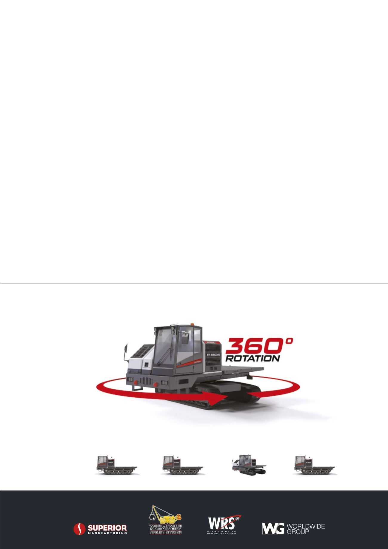
Introducing the New Superior ST-220XR Crawler Carrier
With a 22,000lb payload, swappable cabins and undercarriages, and easy to switch purpose driven beds,
the 220XR turns out quality results for any project.